
Neural networks: tricks of the trade
Pieter-Jan Hoedt @ OPTIMA 2022
@ml_hoedt
;
hoedt@ml.jku.at
Motivation
newcomers to the field waste much time wondering why their networks train so slowly and perform so poorly

Inspiration
Outline
- Data
- Model
- Learning
Outline
- Data
- Model
- Learning
Raw
Data
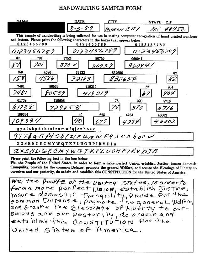
Preprocessed
Data

Looking at
Data
								mean = np.mean(mnist, axis=0)
								plt.imshow(mean)
								plt.show()

								std = np.std(mnist, axis=0)
								plt.imshow(std)
								plt.show()
Looking at
Data
								mean = np.mean(mnist, axis=0)
								plt.imshow(mean, vmin=0, vmax=255, cmap='gray')
								plt.show()

								std = np.std(mnist, axis=0)
								plt.imshow(std, vmin=0, cmap='viridis')
								plt.colorbar()
								plt.show()
Looking at
Data

Looking at
Data

Statistics of the
Data
Transforming
Data


Centred
Data


Normalised
Data


Normalised
Data


PCA-whitened
Data


ZCA-whitened
Data


Why normalise/whiten?
Data
$$\begin{aligned} \mathrm{E}_{\vec{w}} &= \frac{1}{|\mathcal{D}|} \sum_{\vec{x} \in \mathcal{D}} \frac{1}{2} (\vec{w} \cdot \vec{x} - y)^2 \\ \operatorname{\nabla} \mathrm{E}_{\vec{w}} &= \frac{1}{|\mathcal{D}|} \sum_{\vec{x} \in \mathcal{D}} (\vec{w} \cdot \vec{x} - y) \vec{x} \\ \operatorname{\nabla}^2 \mathrm{E}_{\vec{w}} &= \frac{1}{|\mathcal{D}|} \sum_{\vec{x} \in \mathcal{D}} \vec{x} \otimes \vec{x} \end{aligned}$$
Taken from section 5.1 in (LeCun et al., 1998)
Why normalise/whiten?
Data
$\begin{aligned} \mathrm{ E}_{\vec{w}^*} &\approx \mathrm{E}_{\vec{w}} + \operatorname{\nabla} \mathrm{E}_{\vec{w}} \cdot (\vec{w}^* - \vec{w}) \\ %+ \frac{1}{2} \|\vec{w}^* - \vec{w}\|_{\operatorname{\nabla}^2 \mathrm{E}_{\vec{w}}}^2 \\ \operatorname{\nabla} \mathrm{E}_{\vec{w}^*} &\approx \operatorname{\nabla} \mathrm{E}_{\vec{w}} + \operatorname{\nabla}^2 \mathrm{E}_{\vec{w}} \cdot (\vec{w}^* - \vec{w}) \end{aligned}$
$$\vec{w}^* \approx \vec{w} - \bigg(\operatorname{\nabla}^2 \mathrm{E}_{\vec{w}}\bigg)^{-1}\operatorname{\nabla} \mathrm{E}_{\vec{w}}$$
Taken from section 5.1 in (LeCun et al., 1998)
Why not to whiten?
Data

BUT: $\mat{W}_\mathrm{ZCA} = \mat{C}^{-1/2}$
Normalisation of
Data
Practical Normalisation of
Data


Invariances in
Data

TL;DR
Data
- be aware of origins
- gain insights (e.g. using visualisation)
- use statistics to your advantage
- consider inductive biases of the model
Outline
- Data
- Model
- Learning
Baseline
Model
My new hobby is seeing what results I can get on MNIST using k-nearest neighbors. As a baseline kNN gets 96% accuracy without using any special tricks.
— Brandon Rohrer (@_brohrer_) May 25, 2021
96%!
The code:https://t.co/sMAgNuAPiP
k = 5, L1 distance (sum of the absolute value of the difference of the pixel values)
Debugging your
Model
Debugging your
Model
								import numpy as np


								def my_custom_dl_implementation():
									...

Debugging your
Model
								for epoch in range(max_epochs):
									for x, y in train_loader:
										pred = model(x)
										err = loss_func(pred, y)

										opt.zero_grad()
										err.backward()
										opt.step()

									with torch.no_grad():
										for x, y in valid_loader:
											pred = model(x)
											val_err = loss_func(pred, y)

Debugging your
Model
								def update(model, loader, loss_func, opt):
									model.train()

									for x, y in loader:
										pred = model(x)
										err = loss_func(pred, y)

										opt.zero_grad()
										err.backward()
										opt.step()

									return err.item()

								@torch.no_grad()
								def evaluate(model, loader, loss_func):
									model.eval()

									errs = []
									for x, y in loader:
										pred = model(x)
										val_err = loss_func(pred, y)
										errs.append(val_err.item())

									return errs

								val_errs = evaluate(model, valid_loader, loss_func)
								for epoch in range(1, max_epochs + 1):
									err = update(model, train_loader, loss_func, opt)
									val_errs = evaluate(model, valid_loader, loss_func)

Debugging your
Model
Debugging your
Model
								from torch.utils.data import Subset

								if debug:
									train_data = Subset(data, [0, 1])
									valid_data = Subset(data, range(2, len(data)))

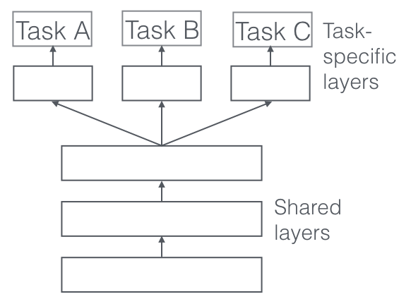
choosing your
Model

Choosing your
Model
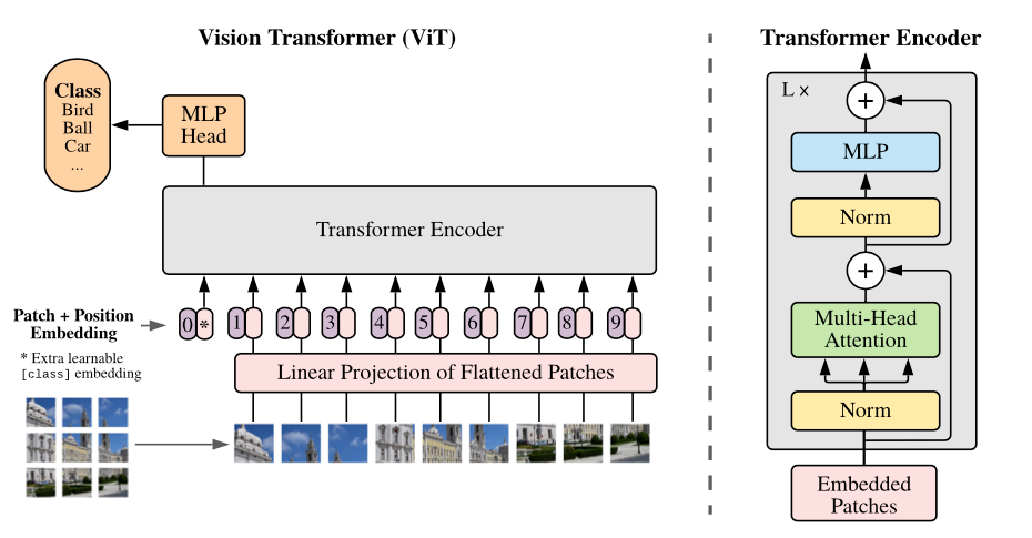
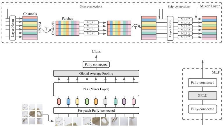
Hopfield networks is all you need (Ramsauer et al., 2021)
choosing your
Model

(van der Smagt & Hirzinger, 1998; Srivasta et al., 2015; He et al., 2016)
Initialising your
Model
- $\sigma_w^2 = \frac{1}{N}$ (Lecun et al., 1998)
- $\sigma_w^2 = \frac{2}{N}$ or $\sigma_w^2 = \frac{2}{M}$ (He et al., 2015)
- $\sigma_w^2 = \frac{2}{N + M}$ (Glorot & Bengio, 2010)
- $\sigma_w^2 = \frac{1}{\sqrt{N M}}$ (Defazio & Bottou, 2021)
Initial biases in your
Model
- Balanced data: $\vec{b} = \vec{0}$
- Unbalanced data: $b_k \propto \ln\Big(\frac{p(y_k)}{1 - p(y_k)}\Big)$
"open" LSTM gate: $\vec{b} \gg 0$
"closed" LSTM gate: $\vec{b} \ll 0$
Normalising your
Model
Batch-normalisation: $$\begin{aligned} \hat{\vec{x}} &= \frac{\vec{x} - \vec{\mu}_\mathcal{B}}{\vec{\sigma}_\mathcal{B}}\\ \vec{y} &= \vec{\gamma} \odot \vec{x} + \vec{\beta} \end{aligned}$$
- before activation function (Ioffe et al., 2015)
- after activation function (Mishkin & Matas, 2016)
Normalising your
Model

Alternatives
- Layer normalisation (Ba et al., 2016)
- Weight normalisation (Salimans & Kingma, 2016)
- Self-normalisation (Klambauer et al., 2017)
- ...
TL;DR
Model
- start as simple as possible
- use prior knowledge (or don't)
- mind the signal flow!
Outline
- Data
- Model
- Learning
Optimisation algorithms
Learning
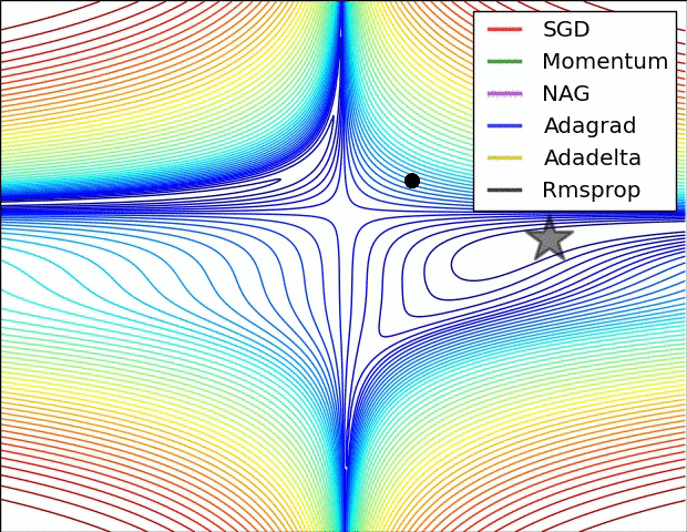
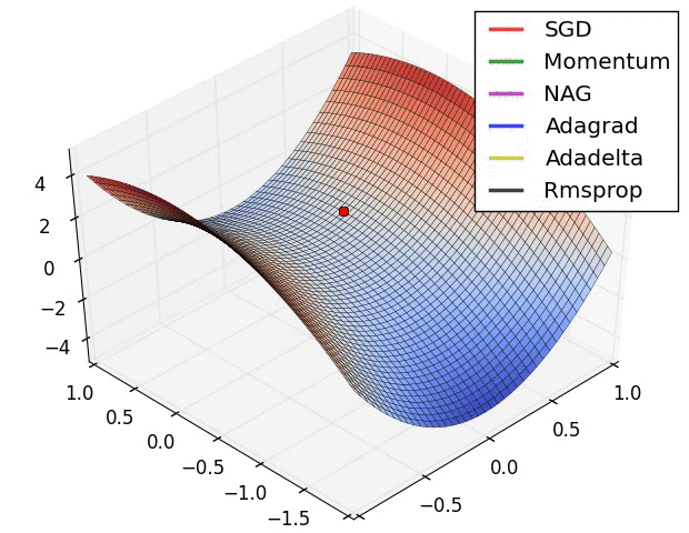
Images from the OG blog post by Sebastian Ruder
Saddle points during
Learning
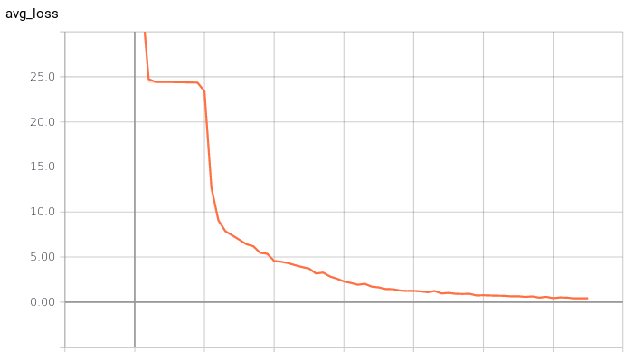
Rate of
Learning

If you have time to tune only one hyperparameter, tune the learning rate.
Deep Learning Book (Goodfellow et al., 2016 )
Rate of
Learning


(Loshchilov & Hutter, 2017; © images from (Zhang et al., 2021))
Rate of
Learning
ce = nn.CrossEntropyLoss(reduction="mean")

Rate of
Learning

ce = nn.CrossEntropyLoss(reduction="sum")
Rate of
Learning

Regularised
Learning
Regularised
Learning

Regularised
Learning
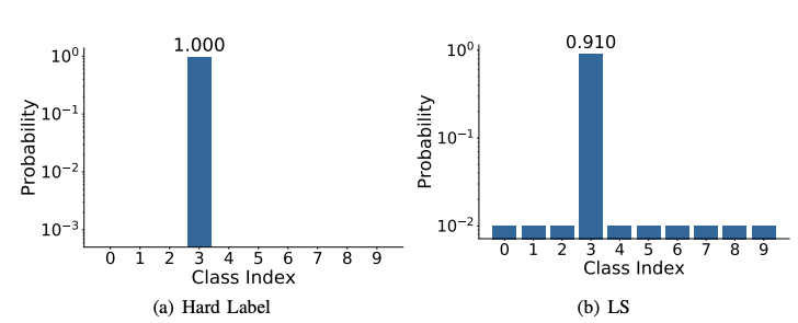

Regularised
Learning

(image taken from wikipedia)
$$\min_\theta L(g(\vec{x} \mathbin{;} \theta), y) + \lambda \|\theta\|$$
(Hanson & Pratt, 1989; Rögnvaldsson, 1998; Loshchchilov & Hutter, 2019)
TL;DR
Learning
- adaptive optimisers are easier (SGD is better)
- maximise the rate of learning
- use regularisation (after overfitting)
TL;DR
- Understand your data
- Keep your model simple
- Learning benefits from tuning
References
Ba et al. (2016). Layer Normalization [Whitepaper]. (link, pdf)
Belkin et al. (2019). Reconciling modern machine-learning practice and the classical bias–variance trade-off. Proceedings of the National Academy of Sciences, 116(32), 15849–15854. (link, pdf)
Bottou et al. (1994). Comparison of classifier methods: A case study in handwritten digit recognition. Proceedings of the 12th IAPR International Conference on Pattern Recognition, 2, 77–82. (link, pdf)
Caruana (1998). A Dozen Tricks with Multitask Learning. In G. B. Orr & K.-R. Müller (Eds.), Neural Networks: Tricks of the Trade (1st ed., pp. 165–191). Springer. (link)
Defazio & Bottou (2021). Beyond Folklore: A Scaling Calculus for the Design and Initialization of ReLU Networks [Preprint]. (link, pdf
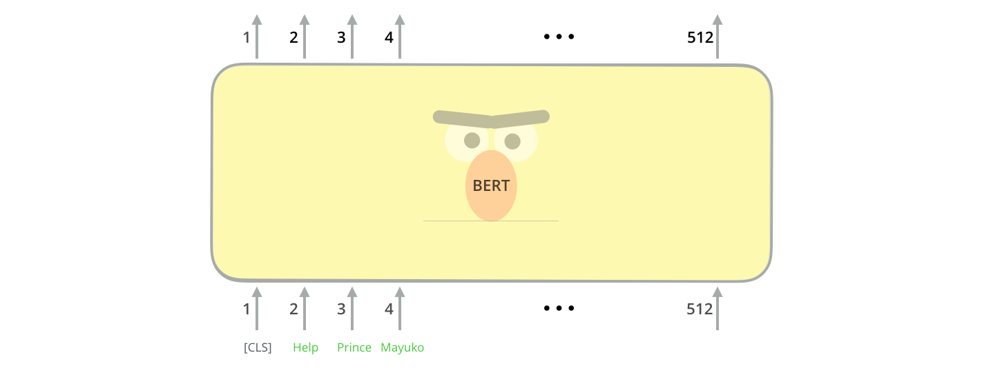
Devlin et al. (2019). BERT: Pre-training of Deep Bidirectional Transformers for Language Understanding. Proceedings of the 2019 Conference of the North American Chapter of the Association for Computational Linguistics: Human Language Technologies, 1, 4171–4186. (link, pdf)
Dosovitskiy et al. (2021). An Image is Worth 16x16 Words: Transformers for Image Recognition at Scale. International Conference on Learning Representations, 9. (link, pdf)
Glorot & Bengio (2010). Understanding the difficulty of training deep feedforward neural networks. Proceedings of the Thirteenth International Conference on Artificial Intelligence and Statistics, 9, 249–256. (link, pdf)
Goodfellow et al. (2016). Deep Learning. MIT Press. (link)
Grother & Hanaoka (1995). Handprinted Forms and Characters Database (Special Database No. 19). National Institute of Standards and Technology. (link, pdf)
Hanson & Pratt (1989). Comparing Biases for Minimal Network Construction with Back-Propagation. Advances in Neural Information Processing Systems, 1, 177–185. (link, pdf)
He et al. (2015). Delving Deep into Rectifiers: Surpassing Human-Level Performance on ImageNet Classification. Proceedings of the IEEE International Conference on Computer Vision, 1026–1034. (link, pdf)
He et al. (2016). Identity Mappings in Deep Residual Networks. In B. Leibe, J. Matas, N. Sebe, & M. Welling (Eds.), Computer Vision – ECCV 2016 (pp. 630–645). Springer International Publishing. (link, pdf)
Hoedt et al. (2022). Normalization is dead, long live normalization!. ICLR Blog Track. (link)
Ioffe & Szegedy (2015). Batch Normalization: Accelerating Deep Network Training by Reducing Internal Covariate Shift. Proceedings of the 32nd International Conference on Machine Learning, 37, 448–456. (link, pdf)
Klambauer et al. (2017). Self-Normalizing Neural Networks. Advances in Neural Information Processing Systems, 30, 971–980. (link, pdf)
LeCun et al. (1998). Efficient BackProp. In G. B. Orr & K.-R. Müller (Eds.), Neural Networks: Tricks of the Trade (1st ed., pp. 9–50). Springer. (link, pdf)
Li et al. (2019). Understanding the Disharmony Between Dropout and Batch Normalization by Variance Shift. 2019 IEEE/CVF Conference on Computer Vision and Pattern Recognition (CVPR), 2677–2685. (link, pdf)
Loshchilov & Hutter (2017). SGDR: Stochastic Gradient Descent with Warm Restarts. International Conference on Learning Representations 5. (link, pdf)
Loshchilov, & Hutter (2018). Decoupled Weight Decay Regularization. International Conference on Learning Representations 6. (link, pdf)
Mishkin et al. (2016). All you need is a good init. International Conference on Learning Representations 4. (link, pdf)
Müller et al. (2019). When does label smoothing help? Advances in Neural Information Processing Systems, 32, 4694–4703. (link, pdf)
Prechelt (1998). Early Stopping—But When? In G. B. Orr & K.-R. Müller (Eds.), Neural Networks: Tricks of the Trade (1st ed., pp. 55–69). Springer. (link, pdf)
Orr & Müller (Eds.). (1998). Neural Networks: Tricks of the Trade (1st ed., Vol. 1524). Springer. (link)
Ramsauer et al. (2021). Hopfield Networks is All You Need. International Conference on Learning Representations 9. (link, pdf)
Rognvaldsson (1998). A Simple Trick for Estimating the Weight Decay Parameter. In G. B. Orr & K.-R. Müller (Eds.), Neural Networks: Tricks of the Trade (1st ed., pp. 71–92). Springer. (link)
Salimans & Kingma (2016). Weight Normalization: A Simple Reparameterization to Accelerate Training of Deep Neural Networks. Advances in Neural Information Processing Systems, 29, 901–909. (link, pdf)
Schraudolph (1998). Centering Neural Network Gradient Factors. In G. B. Orr & K.-R. Müller (Eds.), Neural Networks: Tricks of the Trade (1st ed., pp. 207–226). Springer. (link, pdf)
Srivastava et al. (2014). Dropout: A Simple Way to Prevent Neural Networks from Overfitting. Journal of Machine Learning Research, 15(56), 1929–1958. (link, pdf)
Srivastava et al. (2015). Training Very Deep Networks. Advances in Neural Information Processing Systems, 28, 2377–2385. (link, pdf)
Tolstikhin et al. (2021). MLP-Mixer: An all-MLP Architecture for Vision [Preprint]. (link, pdf)
van der Smagt & Hirzinger (1998). Solving the Ill-Conditioning in Neural Network Learning. In G. B. Orr & K.-R. Müller (Eds.), Neural Networks: Tricks of the Trade (1st ed., pp. 193–206). Springer. (link)
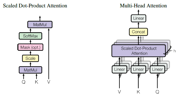
Vaswani et al. (2017). Attention Is All You Need. Advances in Neural Information Processing Systems, 30, 5998–6008. (link, pdf)
Wadia et al. (2021). Whitening and Second Order Optimization Both Make Information in the Dataset Unusable During Training, and Can Reduce or Prevent Generalization. Proceedings of the 38th International Conference on Machine Learning, 139, 10617–10629. (link, pdf)
Wang et al. (2021). Understanding How Dimension Reduction Tools Work: An Empirical Approach to Deciphering t-SNE, UMAP, TriMap, and PaCMAP for Data Visualization. Journal of Machine Learning Research, 22(201), 1–73. (link, pdf)
Wu & He (2018). Group Normalization. In V. Ferrari, M. Hebert, C. Sminchisescu, & Y. Weiss (Eds.), Computer Vision – ECCV 2018 (pp. 3–19). Springer International Publishing. (link, pdf)
Yadav & Bottou (2019). Cold Case: The Lost MNIST Digits. Advances in Neural Information Processing Systems, 32, 13443–13452. (link, pdf)